Hey everyone, and welcome back. In today's video, I'm going to show you an absolutely fantastic package in the R programming language that can make generating residual diagnostic plots an absolute breeze. With just a few lines of code, I will show you how to generate almost every single type of residual diagnostic plot that you could possibly need. If you're ready to stop wasting time generating plots by hand and automate this task, then this is definitely an article you'll want to read.
Getting Started
The first thing we need to generate diagnostic plots on a linear regression model is the linear regression model itself. So we're going to start off by creating a basic linear regression model with the MTCARS data set that comes inbuilt with the R programming language. Obviously, if you are using your own data set, you would pass in the names of the different variables and data set into this function.
head(mtcars)

#This opton uses only selected IVs
model <- lm(mpg~cyl+wt+hp, data = mtcars)

#This model uses ALL cols as IVs
model <- lm(mpg~., data = mtcars)
Just a brief refresher that in the LM function, the first variable, MPG in this case, is the dependent variable, and everything that comes after the squiggly line are the independent variables. If we want to use all of the independent variables, we simply use a period after the squiggly line.
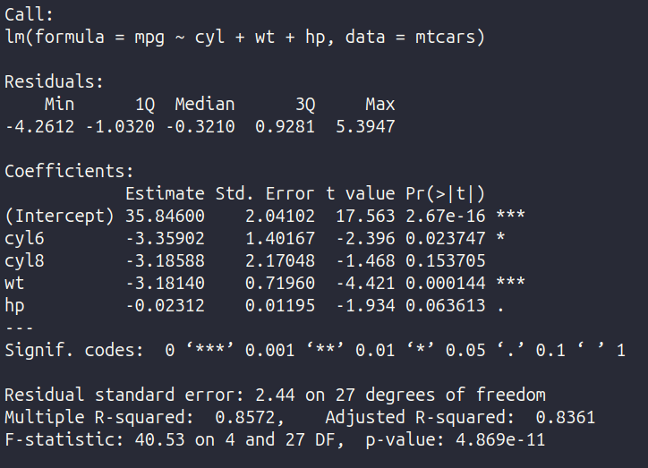
We can then call the summary command on the model to see the basic info such as R squared, F-stat, and the stats for each IV.
summary(model)
Residual Diagnostic Plots
Now that we have our regression model, we can start creating some diagnostic plots. Of course, it is possible to do this in base R using something like a histogram command, but I prefer using the OLSRR package. First, we need to download and install the package with the following commands.
install.packages(olsrr)
library(olsrr)
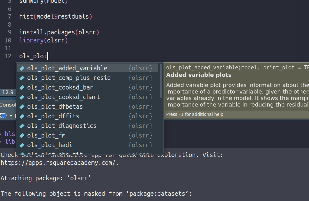
Once the package is pulled into our workspace, we can see all of the available plots by typing olsrr_plot_ and waiting for the dialog to show the selections.
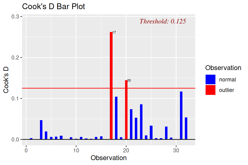
If we just want a single plot, we can easily create it by selecting the right command and passing our model object into the (). For example, the following code creates a Cook's D plot of the model.
ols_plot_cooksd_bar(model)
But Here's The Magic
Although it is possible to create residual plots one at a time, the real magic is the ols_plot_diagnostics() command that automatically creates almost all of the most commonly needed diagnostic plots.
ols_plot_diagnostics(model)
Running the single command above generates each of the following plots.
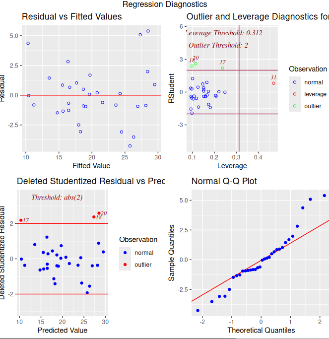
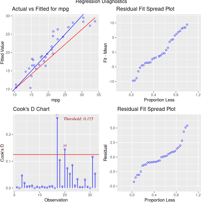
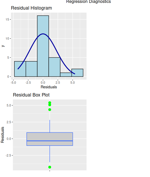
The beauty of this command is that just a single line of code can generate all the plots that we need to assess for heteroscedasticity, normality of residuals, linearity of the relationship, and quickly identify outliers. Obviously, there are times when you might need more advanced plots, but for most of the basics, this will simplify your life so much and save you an incredible amount of time.
Summary
As always, thanks so much for taking the time to read the article. I hope you found it helpful, and I hope you have a super day!