Learn Python Series (#31) - Data Science Part 2 - Pandas
![]()
Repository
- https://github.com/pandas-dev/pandas
- https://github.com/python/cpython
What will I learn?
- You will learn how to convert date/datetime strings into
pandasTimestamps, and set those Timestamp values as index values instead of default integer numbers which don't provide useful context; - how to slice subsets of TimeSeries data using date strings;
- how to slice time-based subsets of TimeSeries data using
.between_time(); - how to return and use some basic statistics based on common
pandasstatistical methods.
Requirements
- A working modern computer running macOS, Windows or Ubuntu;
- An installed Python 3(.7) distribution, such as (for example) the Anaconda Distribution;
- The ambition to learn Python programming.
Difficulty
- Beginner
Curriculum (of the Learn Python Series):
- Learn Python Series - Intro
- Learn Python Series (#2) - Handling Strings Part 1
- Learn Python Series (#3) - Handling Strings Part 2
- Learn Python Series (#4) - Round-Up #1
- Learn Python Series (#5) - Handling Lists Part 1
- Learn Python Series (#6) - Handling Lists Part 2
- Learn Python Series (#7) - Handling Dictionaries
- Learn Python Series (#8) - Handling Tuples
- Learn Python Series (#9) - Using Import
- Learn Python Series (#10) - Matplotlib Part 1
- Learn Python Series (#11) - NumPy Part 1
- Learn Python Series (#12) - Handling Files
- Learn Python Series (#13) - Mini Project - Developing a Web Crawler Part 1
- Learn Python Series (#14) - Mini Project - Developing a Web Crawler Part 2
- Learn Python Series (#15) - Handling JSON
- Learn Python Series (#16) - Mini Project - Developing a Web Crawler Part 3
- Learn Python Series (#17) - Roundup #2 - Combining and analyzing any-to-any multi-currency historical data
- Learn Python Series (#18) - PyMongo Part 1
- Learn Python Series (#19) - PyMongo Part 2
- Learn Python Series (#20) - PyMongo Part 3
- Learn Python Series (#21) - Handling Dates and Time Part 1
- Learn Python Series (#22) - Handling Dates and Time Part 2
- Learn Python Series (#23) - Handling Regular Expressions Part 1
- Learn Python Series (#24) - Handling Regular Expressions Part 2
- Learn Python Series (#25) - Handling Regular Expressions Part 3
- Learn Python Series (#26) - pipenv & Visual Studio Code
- Learn Python Series (#27) - Handling Strings Part 3 (F-Strings)
- Learn Python Series (#28) - Using Pickle and Shelve
- Learn Python Series (#29) - Handling CSV
- Learn Python Series (#30) - Data Science Part 1 - Pandas
Additional sample code files
The full - and working! - iPython tutorial sample code file is included for you to download and run for yourself right here: https://github.com/realScipio/learn-python-series/blob/master/lps-031/learn-python-series-031-data-science-pt2-pandas.ipynb
I've also uploaded to GitHub a CSV file containing all actual BTCUSDT 1-minute ticks on Binance on dates June 2, 2019, June 3, 2019 and June 4, 2019 (4320 rows of actual price data, datetime, open, high, low, close and volume), which file and data set we'll be using:
https://github.com/realScipio/learn-python-series/blob/master/lps-031/btcusdt_20190602_20190604_1min_hloc.csv
GitHub Account
https://github.com/realScipio
Learn Python Series (#31) - Data Science Part 2 - Pandas
Welcome to episode #31 of the Learn Python Series! In the previous episode (Learn Python Series (#30) - Data Science Part 1 - Pandas) I've introduced you to the pandas toolkit, and we've already explained some of the basic mechanisms. In this episode (which is no.2 of the Data Science sub-series, also about pandas) we'll expand our knowledge using more techniques. Let's dive right in!
Time series indexing & slicing techniques using pandas
Analysing actual BTCUSDT financial data using pandas
First, let's download the file btcusdt_20190602_20190604_1min_hloc.csv found here on my GitHub account, and save the file to your current working directory.
Next, let's open the file like so:
import pandas as pd
df = pd.read_csv('btcusdt_20190602_20190604_1min_hloc.csv')
df.head()
| open | high | low | close | volume | datetime | |
|---|---|---|---|---|---|---|
| 0 | 8545.10 | 8548.55 | 8535.98 | 8537.67 | 17.349543 | 2019-06-02 00:00:00+00:00 |
| 1 | 8537.53 | 8543.49 | 8524.00 | 8534.66 | 31.599922 | 2019-06-02 00:01:00+00:00 |
| 2 | 8533.64 | 8540.13 | 8529.98 | 8534.97 | 7.011458 | 2019-06-02 00:02:00+00:00 |
| 3 | 8534.97 | 8551.76 | 8534.00 | 8551.76 | 5.992965 | 2019-06-02 00:03:00+00:00 |
| 4 | 8551.76 | 8554.76 | 8544.62 | 8549.30 | 15.771411 | 2019-06-02 00:04:00+00:00 |
df.shape
(4320, 6)
A quick visual inspection of this CSV file (using .head(), and .shape) shows that we're dealing with a data set consisting of 4320 data rows, and 6 data columns, being datetime, open, high, low, close, and volume.
Nota bene: This data set contains actual trading data of the BTC_USDT trading pair, downloaded from the Binance API, sliced to only contain all 1 minute k-lines / candles on (the example) dates 2019-06-02, 2019-06-03, and 2019-06-04, which I then pre-processed especially for this tutorial episode. The original data returned by the Binance API contains timestamp values in the form of "epoch millis" (milliseconds passed since Jan 1st 1970), and I've converted them into valid ISO-8601 timestamps, which can be easily parsed by the pandas package, as we'll learn in this tutorial.
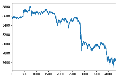
Using the Jupyter Notebook / iPython %matplotlib inline Magic operation, let's take a look how the spot price of Bitcoin has developed minute by minute on these dates, by plotting the df['open'] price values:
%matplotlib inline
df['open'].plot()
Datetime conversion & indexing (using .to_datetime() and .set_index() methods)
The pandas library, while converting the CSV data to a DataFrame object, by default added numerical indexes.
The visual plot example showing the open prices per minute just now, contains X-asis values coming from the numerical indexes that pandas set for now. Although it is clear we're in fact plotting 4320 opening price values, those numbers don't provide any usable context on when the price of Bitcoin was developing over time.
Because we're working with time series now, it would be convenient to be able to set and use the timestamps in the "datetime" column as index values, and to be able to plot those timestamps for visual reference as well.
But if we inspect the data type of the first timestamp (2019-06-02 00:00:00+00:00), by selecting the "datetime" column and the first row (index value 0), like so, we discover that value is now of the string data type:
type(df['datetime'][0])
str
We can convert all "datetime" column values (in one go, with a vectorised column operation) from string objects to pandas Timestamp objects, using the pandas method .to_datetime():
df['datetime'] = pd.to_datetime(df['datetime'])
type(df['datetime'][0])
pandas._libs.tslibs.timestamps.Timestamp
Next, we can re-index the entire DataFrame to not use the default numerical index values, but the converted Timstamp values instead. The .set_index() method is used for this, and calling it will not only use the Timestamps as index values, therewith unlocking a plethora of functionalities, but .set_index() will also remove the 'datetime' column from the data set:
df = df.set_index('datetime')
df.head()
| open | high | low | close | volume | |
|---|---|---|---|---|---|
| datetime | |||||
| 2019-06-02 00:00:00+00:00 | 8545.10 | 8548.55 | 8535.98 | 8537.67 | 17.349543 |
| 2019-06-02 00:01:00+00:00 | 8537.53 | 8543.49 | 8524.00 | 8534.66 | 31.599922 |
| 2019-06-02 00:02:00+00:00 | 8533.64 | 8540.13 | 8529.98 | 8534.97 | 7.011458 |
| 2019-06-02 00:03:00+00:00 | 8534.97 | 8551.76 | 8534.00 | 8551.76 | 5.992965 |
| 2019-06-02 00:04:00+00:00 | 8551.76 | 8554.76 | 8544.62 | 8549.30 | 15.771411 |
Datetime conversion & indexing (using .read_csv() arguments parse_dates= and index_col=)
While reading in the original CSV values from disk, we could have also immediately passed two additional arguments to the .read_csv() method (being: parse_dates= and index_col=), which would have led to the same DataFrame result as we have now:
import pandas as pd
df = pd.read_csv('btcusdt_20190602_20190604_1min_hloc.csv',
                 parse_dates=['datetime'], index_col='datetime')
df.head()
| open | high | low | close | volume | |
|---|---|---|---|---|---|
| datetime | |||||
| 2019-06-02 00:00:00+00:00 | 8545.10 | 8548.55 | 8535.98 | 8537.67 | 17.349543 |
| 2019-06-02 00:01:00+00:00 | 8537.53 | 8543.49 | 8524.00 | 8534.66 | 31.599922 |
| 2019-06-02 00:02:00+00:00 | 8533.64 | 8540.13 | 8529.98 | 8534.97 | 7.011458 |
| 2019-06-02 00:03:00+00:00 | 8534.97 | 8551.76 | 8534.00 | 8551.76 | 5.992965 |
| 2019-06-02 00:04:00+00:00 | 8551.76 | 8554.76 | 8544.62 | 8549.30 | 15.771411 |
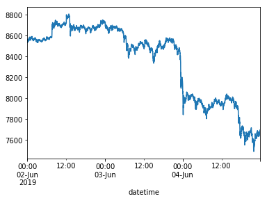
If we again plot these values, now using the DatetimeIndex, our datetime context is plotted on the X-axis as well: nice!
%matplotlib inline
df['open'].plot()
Date slicing
Now that we've successfully set the 'datetime' column as the DataFrame index, we can also slice that index using date strings! If we want to only use a data subset containing 1 day of trading data (= 1440 K-line ticks in this data set), for example on 2019-06-02, then we simply pass the date string as an argument, like so:
df_20190602 = df['2019-06-02']
df_20190602.tail()
| open | high | low | close | volume | |
|---|---|---|---|---|---|
| datetime | |||||
| 2019-06-02 23:55:00+00:00 | 8725.31 | 8728.61 | 8721.67 | 8725.43 | 10.443800 |
| 2019-06-02 23:56:00+00:00 | 8725.45 | 8729.62 | 8720.73 | 8728.66 | 10.184273 |
| 2019-06-02 23:57:00+00:00 | 8728.49 | 8729.86 | 8724.37 | 8729.10 | 10.440185 |
| 2019-06-02 23:58:00+00:00 | 8729.05 | 8731.14 | 8723.86 | 8723.86 | 9.132625 |
| 2019-06-02 23:59:00+00:00 | 8723.86 | 8726.00 | 8718.00 | 8725.98 | 9.637084 |
As you can see on the .tail()output, the last DataFrame row of the newly created df_20190602 DataFrame is 2019-06-02 23:59:00, and the df_20190602 DataFrame only contains 1440 rows of data in total:
df_20190602.shape
(1440, 5)
In case we want to create a DataFrame containing a multiple day window subset, we also add a stop date to the date string slice, like so:
df_20190602_20190603 = df['2019-06-02':'2019-06-03']
df_20190602_20190603.tail()
| open | high | low | close | volume | |
|---|---|---|---|---|---|
| datetime | |||||
| 2019-06-03 23:55:00+00:00 | 8170.31 | 8178.48 | 8162.61 | 8169.20 | 46.913377 |
| 2019-06-03 23:56:00+00:00 | 8169.24 | 8175.39 | 8159.00 | 8161.52 | 44.748378 |
| 2019-06-03 23:57:00+00:00 | 8161.16 | 8161.17 | 8135.94 | 8146.69 | 65.794209 |
| 2019-06-03 23:58:00+00:00 | 8146.58 | 8153.00 | 8137.38 | 8140.00 | 43.648000 |
| 2019-06-03 23:59:00+00:00 | 8140.00 | 8142.80 | 8100.50 | 8115.82 | 185.607380 |
df_20190602_20190603.shape
(2880, 5)
Nota bene: It's important to note that - unlike on "regular" (index) slicing, - when using date string slicing in pandas both lower and upper boundaries are inclusive; the data being sliced includes all 1440 data rows from June 3, 2019.
Time slicing using .between_time()
What if we want to slice all 1-minute candles which happened one a specific day (e.g. on 2019-06-02) between a specific time interval, for example between 14:00 UTC and 15:00 UTC? This we can accomplish using the .between_time() method.
As arguments, we pass the arguments start_time, end_time, and we specify include_end=False so that the end_time is non-inclusive (if we wouldn't, our new sub-set would include 61 instead of 60 1-minute ticks).
df_20190602_1h = df_20190602.between_time('14:00', '15:00', include_end=False)
df_20190602_1h.tail()
| open | high | low | close | volume | |
|---|---|---|---|---|---|
| datetime | |||||
| 2019-06-02 14:55:00+00:00 | 8665.71 | 8669.50 | 8663.66 | 8667.24 | 11.401655 |
| 2019-06-02 14:56:00+00:00 | 8668.06 |