~~~ La versione in italiano inizia subito dopo la versione in inglese ~~~
ENGLISH

22-09-2025 - Operations Research - LP Exercise [EN]-[IT] With this post, I would like to provide a brief instruction on the topic mentioned above. (lesson/article code: MS_11)

image created with artificial intelligence, the software used is Microsoft Copilot
Introduction Today I'll try to demonstrate a linear programming exercise. Linear programming is a discipline that was born about 60 years ago; it didn't exist before. Linear programming helps decision-making by examining the problem from three main perspectives: the objective function, the constraints, and the variables. It is used to solve problems in industrial planning or manufacturing.
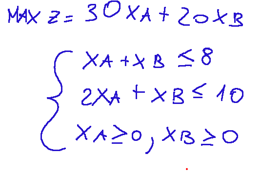
Exercise Let's imagine a factory produces two parts called A and B. A's profit is €30 B's profit is €20
We then have two assembly departments, R1 and R2. R1 spends 1 hour on the production of parts A and 1 hour on B, working 8 hours a day. R2 spends 2 hours on the production of parts A and 1 hour on B, working 10 hours a day.
At this point, we transform the problem mathematically by identifying the objective function and the various constraints.
The Graphical Method To understand the optimum, that is, the best solution given the given constraints, we need to plot the lines that make up the graph, and their intersection will be the optimal point.
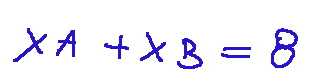
Let's consider the first constraint, which I report below:

Let's translate this constraint into an equality, which would be the boundary of the inequality.
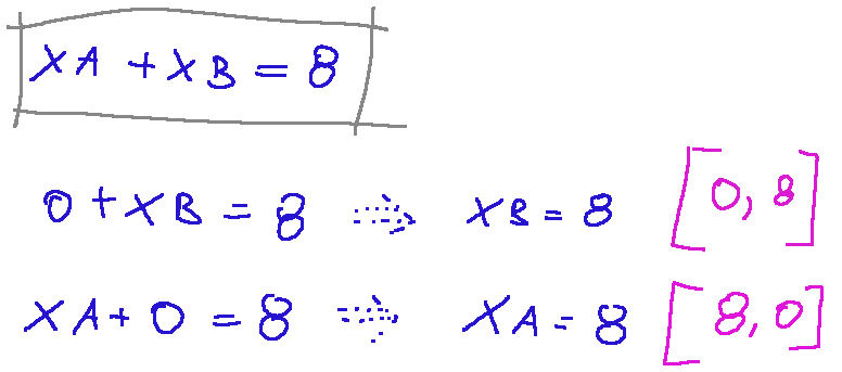
Now let's set the two variables xA and xB to zero, first one and then the other, to calculate the two points through which the first line will pass. We will have the following.
Now let's do the same operation with the second constraint of the problem.
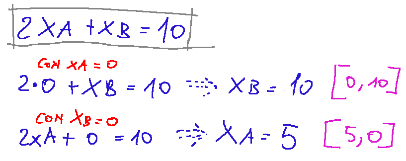
Construction of the graph For the first constraint, that of xA+xB<=8, I will have a straight line that passes through the following points: [8,0] [0,8] For the second constraint, 2xA+xB<=10, I will have a line that passes through the following points: [5,0] [0,10]
Here's what happens if we now plot the graph.
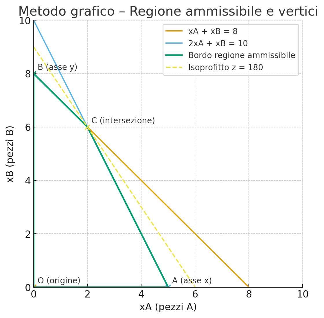
image created with artificial intelligence, the software used is ChatGPT
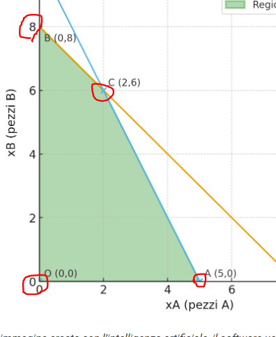
The orange line represents the first constraint and the blue line represents the second constraint. The intersection C, i.e., the point [2,6], represents the optimum, or the optimal solution.
The feasible region
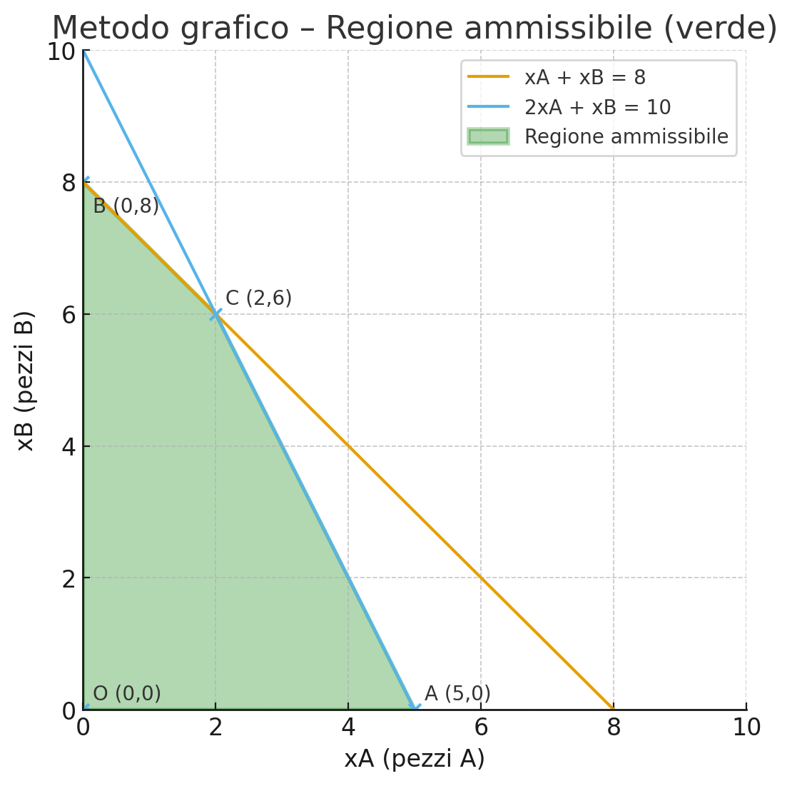
Image created with artificial intelligence, the software used is ChatGPT
The green area I colored is the set of all combinations (xA,xB) that satisfy both constraints, and this area is called the feasible region
Intersection of the two lines To verify the intersection of the two lines, we can solve the system of equations. I've reproduced the system of equations below.
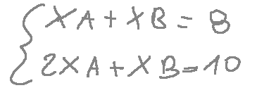
I solve the system using the substitution method.
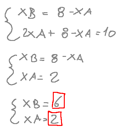
So we've verified that intersection C is (2,6)
Considerations Let's evaluate the objective at vertices 0, A, B, and C, remembering that: A's profit is €30 B's profit is €20
At 0, at z(0,0), the profit is 0 At A, at z(5,0), the profit is €150 At B, at z(0,8), the profit is €160 At C, at z(2,6), the profit is €180, the maximum
Result The The optimal solution is the following.

Conclusions Linear programming is used to transform technical data into optimal decisions. It will help the company make the

ITALIAN

22-09-2025 - Ricerca operativa - Esercizio di PL [EN]-[IT] Con questo post vorrei dare una breve istruzione a riguardo dell’argomento citato in oggetto (codice lezione/articolo: MS_11)
immagine creata con l’intelligenza artificiale, il software usato è Microsoft Copilot
Introduzione Oggi provo a mostrare un esercizio di programmazione lineare. La programmazione lineare è una disciplina nata circa 60 anni fa, prima non esisteva. La programmazione lineare aiuta a prendere decisioni esaminando il problema da tre punti di vista principali. La funzione obiettivo, i vincoli e le variabili. Viene usata per risolvere problemi nella pianificazione industriale o nella produzione industriale.
Esercizio Immaginiamo che una fabbrica produca due pezzi che si chiamano A e B. Il profitto di A è di 30€ Il profitto di B è di 20€
Abbiamo poi due reparti di montaggio R1 e R2 R1 impiega per la produzione dei pezzi: 1h per A e 1h per B e lavora 8 ore al giorno R2 impiega per la produzione dei pezzi: 2h per A e 1h per B e lavora 10 ore al giorno
A questo punto trasformiamo matematicamente il problema identificando la funzione obiettivo e i vari vincoli.
Il metodo grafico Per capire qual è l'ottimo, cioè qual è la soluzione migliore in base ai vincoli dati, dobbiamo tracciare le rette che compongono il grafico e la loro intersezione sarà il punto ottimale.
Prendiamo in considerazione il primo vincolo che riporto qui sotto:
Portiamo questo vincolo in forma di eguaglianza che sarebbe il bordo della disuguaglianza.
Ora portiamo le due variabili xA e xB a zero, prima l'una e poi l'altra per calcolare i due punti da cui passerà la prima retta. Avremo quanto segue.
Ora facciamo la stessa operazione con il secondo vincolo del problema
Costruzione del grafico Per il primo vincolo quello di xA+xB<=8 avrò una retta che passa per i seguenti punti: [8,0] [0,8] Per il secondo vincolo quello di 2xA+xB<=10 avrò una retta che passa per i seguenti punti: [5,0] [0,10]
Ecco che cosa succede se ora andiamo a tracciare il grafico
immagine creata con l’intelligenza artificiale, il software usato è ChatGPT
LA retta arancione rappresenta il primo vincolo e la retta azzurra rappresenta il secondo vincolo. L'intersezione C, cioè il punto [2,6] rappresenta l'ottimo ovvero la soluzione ottima
La regione ammissibile
immagine creata con l’intelligenza artificiale, il software usato è ChatGPT
L'area verde che ho fatto colorare è l'insieme di tutte le combinazioni (xA,xB) che rispettano entrambi i vincoli e questa zona viene chiamata, regione ammissibile
Intersezione delle due rette Per verificare l'intersezione delle due rette possiamo risolvere il sistema di equazioni. Riporto il sistema di equazioni qui sotto
Risolvo il sistema con il metodo della sostituzione
Così abbiamo verificato che l'intersezione C è (2,6)
Considerazioni valutiamo l'obiettivo sui vertici 0, A, B e C ricordando che: Il profitto di A è di 30€ Il profitto di B è di 20€
in 0 avremo che z(0,0) il profitto è 0 in A avremo che z(5,0) il profitto è 150€ in B avremo che z(0,8) il profitto è 160€ in C avremo che z(2,6) il profitto è 180€ il massimo
Risultato La soluzione ottima è la seguente
Conclusioni La programmazione lineare serve per trasformare dati tecnici in decisioni ottime. Essa aiuterà l'azienda a prendere la decisione migliore nell'ambito della produzione.
Domanda La programmazione lineare, oltre a risolvere problemi come quello proposto in questo post, risolve problemi di logistica. Lo sapevate che anche Amazon si avvale della programmazione lineare per gestire i magazzini e le rotte di consegna? Sapevate che in questo modo Amazon riduce i tempi e i costi operativi?
THE END