~~~ La versione in italiano inizia subito dopo la versione in inglese ~~~
ENGLISH

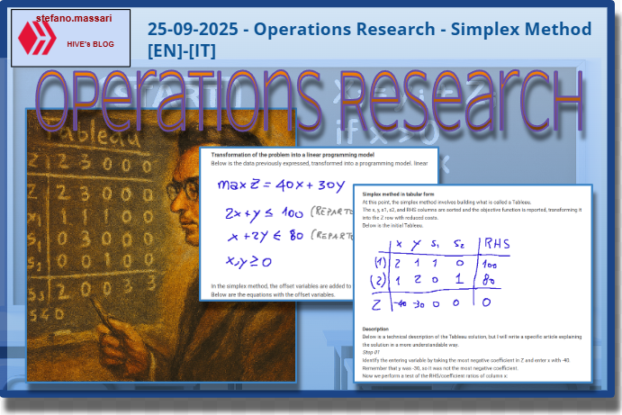
25-09-2025 - Operations Research - Simplex Method [EN]-[IT] With this post, I would like to provide a brief introduction to the topic in question. (lesson/article code: MS_12)
Image created with artificial intelligence, the software used is Microsoft Copilot
Introduction The simplex method is an algorithm used in linear programming to solve problems with many variables. This method is based on the following: - Verification of the optimality criterion - Verification of the unboundedness criterion - Identification of a new feasible basic solution
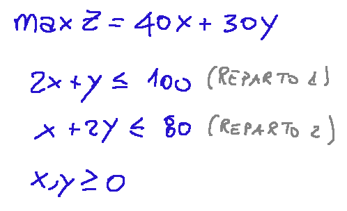
Example Let's try an example with just two products, A and B, manufactured by two departments, 1 and 2, with the following data: A, with a cost of €40 per unit, requires 2 hours in department 1 and 1 hour in department 2 B, with a cost of €30 per unit, requires 1 hour in department 1 and 2 hours in department 2
Availability hours for each department: Department 1 is active for 100 hours Department 2 is active for 80 hours
Transformation of the problem into a linear programming model Below is the data previously expressed, transformed into a programming model. linear
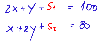
In the simplex method, the offset variables are added to the equation. Below are the equations with the offset variables.
Simplex method in tabular form At this point, the simplex method involves building what is called a Tableau. The x, y, s1, s2, and RHS columns are sorted and the objective function is reported, transforming it into the Z row with reduced costs. Below is the initial Tableau.
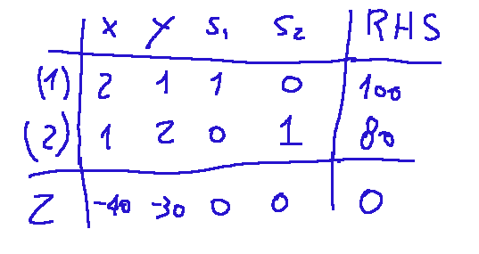
Description Below is a technical description of the Tableau solution, but I will write a specific article explaining the solution in a more understandable way. Step 01 Identify the entering variable by taking the most negative coefficient in Z and enter x with -40. Remember that y was -30, so it was not the most negative coefficient. Now we perform a test of the RHS/coefficient ratios of column x: So: In row 1 we have 100/2=50 In row 2 we have 80/1=80
Step 02 Let's normalize row 1 by dividing by 2, which becomes: 1 --> [1, 0.5, 0.5, 0 ∣ 50]
Then we set column x in the second department row and Z to zero, so we have
(2) --> (2)-(1) --> [0, 1.5, -0.5, 1 ∣ 30] Z --> Z+40*(1) --> [0, -10, 20, 0 ∣ 2200]
Step 03 We calculate the entering variable and we will have that in Z -10 remains negative on y --> enters y Normalizing row 2 We will have: (2) --> [0, 1, -1/3, 2/3 ∣ 20]
Resetting column Y to zero leaves: (1) = (1)-0.5(2) --> [1, 0, 2/3, -1/3 ∣ 40] Z = Z+10*(2) --> [0, 0, 50/3, 20/3 ∣ 2200]
Now there are no negative coefficients in row Z, which means that the optimum has been reached.
Optimal Solution x=40 y=20
Conclusions With the given constraints, namely 2x+y<=100 and x+2y<=80, the simplex method yields the optimum at two points: Produce A=40 and B=20, with a maximum margin of €2,200 and fully saturated departments. This is an exceptional method for solving company production and cost problems.
Question Have you ever heard of the simplex method? Did you know that this algorithm for finding the best solution to a linear programming problem was invented by American mathematician and statistician George Bernard Dantzig in 1947? Did you know that in the 1950s, this method was used to calculate optimal fuel mixtures?

ITALIAN

25-09-2025 - Ricerca operativa - Metodo del Simplesso [EN]-[IT] Con questo post vorrei dare una breve istruzione a riguardo dell’argomento citato in oggetto (codice lezione/articolo: MS_12)
immagine creata con l’intelligenza artificiale, il software usato è Microsoft Copilot
Introduzione Il metodo del simplesso è un algoritmo che viene usato in programmazione lineare per risolvere i problemi con molte variabili. Questo metodo si basa sulle seguenti cose: -verifica del criterio di ottimalità -verifica del criterio di illimitatezza -identificazione di una nuova soluzione di base ammissibile
Esempio Proviamo a fare un esempio con solo due prodotti A e B, costruiti da due reparti 1 e 2 con i seguenti dati: A con costo 40€ a pezzo, richiede 2h nel reparto 1 e 1h nel reparto 2 B con costo 30€ a pezzo, richiede 1h nel reparto 1 e 2h nel reparto 2
Disponibilità ore per ogni reparto: Il Reparto 1 è attivo per 100h Il reparto 2 è attivo per 80h
Trasformazione del problema in un modello di programmazione lineare Qui di seguito i dati prima espressi trasformati in un modello di programmazione lineare
Nel metodo del simplesso si usa aggiungere le variabili si scarto all'equazione Qui di seguito le equazioni con le variabili di scarto.
Metodo del simplesso in forma tabellare A questo punto il metodo del simplesso prevede di costruire quello che viene chiamato Tableau. Vengono ordinate le colonne x,y,s1,s2, RHS e si riporta la funzione obiettivo trasformandola nella riga Z con costi ridotti. Qui di seguito il Tableau iniziale
descrizione Qui di seguito una descrizione tecnica della risoluzione del Tableau, ma provvederò a fare un articolo specifico proprio sulla spiegazione della risoluzione di un Tableau in maniera più comprensibile. Passo 01 Si individua la variabile entrante prendendo il coefficiente più negativo in Z ed entra x con -40, ricordiamo che y era -30, quindi non era il coefficiente più negativo. Ora si effettua un test dei rapporti RHS/coefficienti colonna x: Quindi: in riga 1 abbiamo 100/2=50 in riga 2 abbiamo 80/1=80
Passo 02 Andiamo a normalizzare la riga 1 dividendo per 2 che diventerà: 1 --> [1, 0.5, 0.5, 0 ∣ 50]
Poi azzeriamo la colonna x nella riga del secondo reparto e Z, avremo così
(2) --> (2)-(1) --> [0, 1.5, -0.5, 1 ∣ 30] Z --> Z+40*(1) --> [0, -10, 20, 0 ∣ 2200]
Passo 03 Calcoliamo la variabile entrante e avremo che in Z rimane negativo -10 su y --> entra y Normalizzando la riga 2 avremo: (2) --> [0, 1, -1/3, 2/3 ∣ 20]
Azzerando la colonna Y rimarrà: (1) = (1)-0.5(2) --> [1, 0, 2/3, -1/3 ∣ 40] Z = Z+10*(2) --> [0, 0, 50/3, 20/3 ∣ 2200]
Ora nella riga Z non ci sono coefficienti negativi questo significa che l'ottimo è stato raggiunto
Soluzione ottima x=40 y=20
Conclusioni Con i vincoli dati cioè 2x+y<=100 e x+2y<=80 il metodo del simplesso porta all’ottimo in due punti: produrre A=40 e B=20, con margine massimo 2200 € e reparti completamente saturi. Questo è un metodo eccezionale per risolvere problemi di produzione aziendale e di costi aziendali.
Domanda Avete mai sentito parlare del metodo de simplesso? Sapevate che questo algoritmo per trovare la soluzione migliore ad un problema di programmazione lineare fu inventato dal matematico e statistico statunitense George Bernard Dantzig nel 1947? Sapevate che negli anni 50 con questo metodo venivano calcolate le miscele ottimali dei carburanti?
THE END