
~~~ La versione in italiano inizia subito dopo la versione in inglese ~~~
ENGLISH

27-09-2025 - Applied Mechanics - Friction [EN]-[IT] With this post, I would like to provide a brief introduction to the topic mentioned above. (lesson/article code: LE_90)

Image created with artificial intelligence, the software used is Microsoft Copilot
Introduction Applied mechanics is a branch of engineering that studies the behavior of real mechanical devices, using the principles of theoretical mechanics. In applied mechanics, studies involving friction are very important. In physics, friction is the resisting force that opposes the motion of an object or its displacement on a surface.
The various types of friction
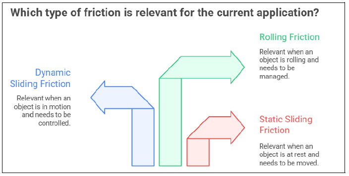
Image created with artificial intelligence, the software used is Napkin.ai
There are three main types of friction. Sliding friction – static Sliding friction – dynamic Rolling friction
Sliding friction – static Static sliding friction can be defined as the force that opposes the initiation of motion between two surfaces in contact. The formula for static friction is shown below.
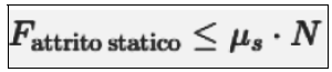
Where: μs = coefficient of static friction N = normal force between surfaces. Please note that the maximum value of static friction is that which occurs just before motion begins.
Sliding Friction – Dynamic Case Dynamic sliding friction is also called kinetic sliding friction and is the force that opposes relative motion when the body is already in motion.
The formula has a slight variation from that for static sliding friction and is shown below.
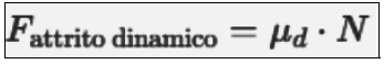
Where: μd = coefficient of kinetic friction, usually μd < μs N = constant force acting in the direction opposite to the motion.
Rolling friction Rolling friction is the friction that exists when a body rolls on a surface. This type of friction, unlike the two previous ones described above, is not a force, but a resisting torque or an equivalent force that opposes rolling. This friction depends on the deformation of the surfaces (think of a wheel on a road) and the internal resistance of the materials. Below is the formula for rolling friction;
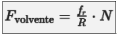
Where: fr = coefficient of rolling friction R = radius of the rolling body
Dynamic diagram of a driven roller A roller that does not receive a driving torque, but moves under the effect of an external force, is called a driven roller. The figure below highlights what we can define as driven rollers. Below is a diagram showing what we define as driven rollers.
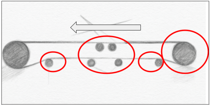
In this case, the dynamic equilibrium equations are as follows: Translational equilibrium:
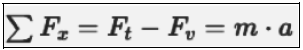
Where: Fv = Rolling friction force Ft = Rolling friction force drag Rotational equilibrium:
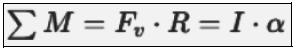
Where: I = moment of inertia α = angular acceleration
Dynamic diagram of a drive roller A roller that, unlike the previous one, receives a driving torque and transmits motion is called a drive roller. Below is a diagram showing what is called the drive roller.
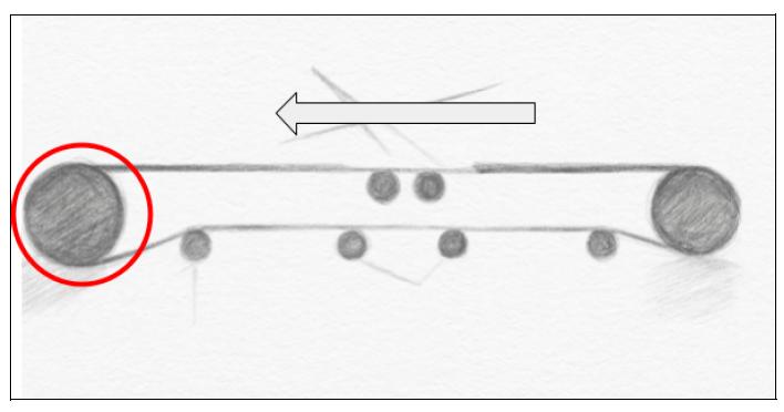
In this case, the dynamic equilibrium equations are as follows:
Translational equilibrium
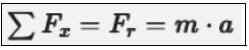
Where: Fr = force Reaction Rotational Equilibrium
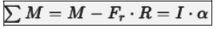
Where: M = Drive torque
Conclusions We can summarize the concept of friction by saying that it is a force that opposes motion and can exist and act both when the body is stationary and when it is in motion. Friction arises from microscopic irregularities in surfaces, intermolecular forces, and deformations of materials. An example of friction is the friction between the brake pads and the disc of a vehicle, which is used to brake a car. Another example of friction is that between belts and pulleys; in this case, friction enables the transmission of motion.
Question Did you know that the Italian scientist, inventor, and artist Leonardo Da Vinci (1452–1519) is considered one of the first scientists to scientifically study friction? Did you know that in his manuscripts, he observed that frictional force is proportional to the applied load and that friction is independent of the contact area between surfaces?

ITALIAN

27-09-2025 - Meccanica Applicata - Gli attriti [EN]-[IT] Con questo post vorrei dare una breve istruzione a riguardo dell’argomento citato in oggetto (codice lezione/articolo: LE_90)
immagine creata con l’intelligenza artificiale, il software usato è Microsoft Copilot
Introduzione La meccanica applicata è una branca dell’ingegneria che studia il comportamento dei dispositivi meccanici reali, utilizzando i principi della meccanica teorica. Nella meccanica applicata gli studi che riguardano gli attriti sono molto importanti. L’attrito in fisica è quella forza resistente che si oppone al movimento di un oggetto o al suo spostamento sulla superficie.
Le varie tipologie di attrito
immagine creata con l’intelligenza artificiale, il software usato è Napkin.ai
Abbiamo tre principali tipologie di attrito. Attrito radente – caso statico Attrito radente – caso dinamico Attrito volvente
Attrito radente – caso statico L’attrito radente statico possiamo definirlo come la forza che si oppone all’inizio del moto tra due superfici a contatto. Qui di seguito è rappresentata la formula dell’attrito statico
Dove: μs = coefficiente di attrito statico N = forza normale tra le superfici. Si precisa che Il valore massimo dell’attrito statico è quello che si verifica appena prima che inizi il moto.
Attrito radente – caso dinamico L’attrito radente dinamico viene anche chiamato attrito radente cinetico ed è la forza che si oppone al moto relativo quando il corpo è già in movimento. La formula ha una piccola variazione rispetto a quella dell’attrito radente statico ed è riportata qui di seguito.
Dove: μd = coefficiente di attrito dinamico, solitamente μd < μs N = forza costante che agisce in direzione opposta al moto.
Attrito radente volvente L’attrito volvente è l’attrito che esiste quanto un corpo rotola su una superficie. Questa tipologia di attrito,differentemente dalle due precedenti descritte sopra, non è una forza, ma una coppia resistente o una forza equivalente che si oppone al rotolamento. Questo attrito dipende dalla deformazione delle superfici (pensiamo ad una ruota su strada) e dalla resistenza interna dei materiali. Qui di seguito la formula dell’attrito volvente;
Dove: fr = coefficiente di attrito volvente R = raggio del corpo rotolante
Schematizzazione dinamica di un rullo trainato Un rullo che non riceve una coppia motrice, ma si muove per effetto di una forza esterna si definisce rullo trainato Nella figura qui sotto sono evidenziati quelli che possiamo definire rulli trainati. Qui di seguito uno schema dove sono segnati quelli che vengono definiti rulli trainati.
In questo caso le equazioni di equilibrio dinamico sono le seguenti: Equilibrio traslazionale:
Dove: Fv = Forza di attrito volvente Ft = Forza di trascinamento
Equilibrio rotazionale
Dove: I = momento d’inerzia α = accelerazione angolare
Schematizzazione dinamica di un rullo motore Un rullo che, al contrario di prima, riceve una coppia motrice e trasmette del moto, si definisce rullo motore. Qui di seguito uno schema dove sono segnati quelli che viene definito rullo motore
In questo caso le equazioni di equilibrio dinamico sono le seguenti:
Equilibrio traslazionale
Dove: Fr = forza di reazione Equilibrio rotazionale
Dove: M = Coppia motrice
Conclusioni Possiamo sintetizzare il concetto di attrito dicendo che è una forza che si oppone al movimento e può esistere agire sia quando il corpo è fermo sia quando è in movimento. Gli attriti derivano dalle irregolarità microscopiche delle superfici, dalle forze intermolecolari e dalle deformazioni dei materiali. Un esempio di attrito può essere quello che c’è tra le pastiglie e il disco di un veicolo, attrito che serve per frenare un’auto. Un altro esempio di attrito è quello che avviene tra cinghie e pulegge, in questo caso l’attrito consente la trasmissione del moto.
Domanda Sapevate che lo scienziato, inventore e artista italiano, Leonardo Da Vinci (1452 – 1519) è considerato uno dei primi scienziati che ha fatto studi sull’attrito in modo scientifico? Sapevate che nei suoi manoscritti ha osservato che la forza di attrito è proporzionale al carico applicato e che l’attrito è indipendente dall’area di contatto tra le superfici?
THE END