The end of the year is always a catastrophe in terms of availability. University duties are heavy, with exams and a decent amount of administration. Moreover, my health is still not great, and issues are piling up on top of each other. Having got COVID at a scientific conference a month ago changed my life quite badly.
For that reason, my on-chain presence is kind of reduced, both for STEMsocial, my own blog and all projects I run here. However, I am never very far and things get eventually done!
Today, I decided to go back to the citizen science project that we started a couple of months ago. This project focuses on a particle physics study of a neutrino mass model at CERN’s Large Hadron Collider (aka the LHC), and the key point is that non-scientific actors from the Hive community will conduct it (under my guidance). I recently wrote a blog on the general context behind this study, that can be found here.
The topic of the present episode concerns the simulation of the neutrino signal that we aim to study. We will first make sure that every participant is comfortable in using the tools we installed a while ago. For this purpose, we plan to reproduce some results from a scientific publication from 2020. In a second stage, those older results will be extended to a situation that has never been considered so far.
In other words, we plan to produce brand new scientific results on Hive!
 [Credits: geralt (Pixabay)]
Let’s start with a recap of the previous episodes of our adventure. This should allow anyone motivated in joining us to catch up. In terms on involvement, a couple of hours by episode are in principle sufficient.
[Credits: geralt (Pixabay)]
Let’s start with a recap of the previous episodes of our adventure. This should allow anyone motivated in joining us to catch up. In terms on involvement, a couple of hours by episode are in principle sufficient.
 [Credits: @lemouth]
If yes, then you are ready to simulate our signal beyond the Standard Model of particle physics.
---
[Credits: @lemouth]
If yes, then you are ready to simulate our signal beyond the Standard Model of particle physics.
---
 [Credits: CMS-EXO-21-003 (CMS @ CERN)]
Our two quarks carry a lot of energy, as their associated protons are accelerated close to the speed of light. Moreover, these quarks are sensitive to weak interactions. As a consequence, each of them has a given probability to emit a W boson, one of the mediators of the weak interactions. Those two W bosons are given in purple in the figure.
What comes next is the interesting part of our new physics process. The two W bosons exchange a heavy neutrino N, in red in the figure, and this leads to the production of two leptons of the same electric charge (see the symbols l1 and l2 on the right part of the figure).
The process described above is precisely the signal that we want to simulate. It depends on one of the new particles of the model N (one of the included heavy neutrinos), and on its properties (how it couples to electrons, muons and taus).
In the reference scientific publication, my collaborators and I studied the production of two muons or two antimuons. In the study that is planned to be conducted on Hive, we will consider all other possibilities (pairs of electrons, pairs of taus, mixed pairs of different leptons, etc.).
For today, however, we want to make sure everybody uses MG5aMC for new physics simulations correctly. For this reason, we consider the production of muons as in the 2020 publication, and aim at reproducing some of the results shown in that article.
---
[Credits: CMS-EXO-21-003 (CMS @ CERN)]
Our two quarks carry a lot of energy, as their associated protons are accelerated close to the speed of light. Moreover, these quarks are sensitive to weak interactions. As a consequence, each of them has a given probability to emit a W boson, one of the mediators of the weak interactions. Those two W bosons are given in purple in the figure.
What comes next is the interesting part of our new physics process. The two W bosons exchange a heavy neutrino N, in red in the figure, and this leads to the production of two leptons of the same electric charge (see the symbols l1 and l2 on the right part of the figure).
The process described above is precisely the signal that we want to simulate. It depends on one of the new particles of the model N (one of the included heavy neutrinos), and on its properties (how it couples to electrons, muons and taus).
In the reference scientific publication, my collaborators and I studied the production of two muons or two antimuons. In the study that is planned to be conducted on Hive, we will consider all other possibilities (pairs of electrons, pairs of taus, mixed pairs of different leptons, etc.).
For today, however, we want to make sure everybody uses MG5aMC for new physics simulations correctly. For this reason, we consider the production of muons as in the 2020 publication, and aim at reproducing some of the results shown in that article.
---
 [Credits: @lemouth]
Feel free to click on a few
[Credits: @lemouth]
Feel free to click on a few 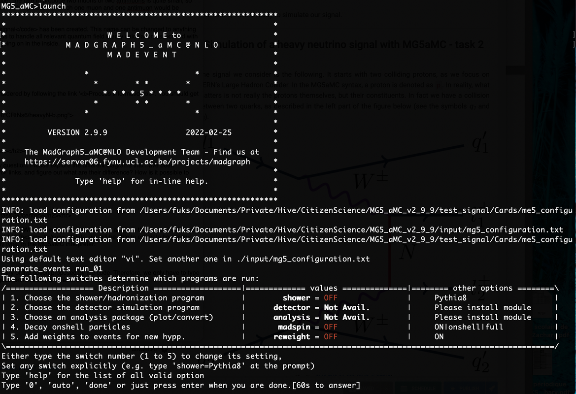 [Credits: @lemouth]
Next, MG5aMC asks us whether we want to modify the parameters of the model (the
[Credits: @lemouth]
Next, MG5aMC asks us whether we want to modify the parameters of the model (the
[Credits: geralt (Pixabay)]
Let’s start with a recap of the previous episodes of our adventure. This should allow anyone motivated in joining us to catch up. In terms on involvement, a couple of hours by episode are in principle sufficient.
- Episode 1 was about the installation of the MG5aMC software dedicated to particle collider simulations. We got seven reports from the participants (agreste, eniolw, gentleshaid, mengene, metabs, servelle and travelingmercies), among which that of @metabs consists of an excellent documentation on how to get started with a virtual machine running on Windows.
- In episode 2 we made use of MG5aMC to generate 10,000 simulated LHC collisions relative to the production of a top-antitop pair at the LHC. We got eight reports from the participants (agreste, eniolw, gentleshaid, isnochys, mengene, metabs, servelle and travelingmercies).
- Episode 3 focused on the installation of MadAnalysis5, a piece of software allowing us to simulate detector effects, reconstruct the output of complex simulations, and the analysis of produced events. We got seven contributions (agreste, eniolw, gentleshaid, isnochys, metabs, servelle and travelingmercies).
- Episode 4 was a study of top-antitop production at CERN’s Large Hadron Collider. We got five contributions (agreste, eniolw, gentleshaid, servelle and travelingmercies). The solutions to the proposed assignments are available here.
Signal and background at the LHC
--- In the previous episodes of our citizen science project on Hive, we have used quite a bit the simulation software MG5aMC. All the simulations done so far however relies on the Standard Model of particle physics. This is not what we aim to do in our project targeting the simulation of a signal of a new phenomenon. Of course, we will have to deal with Standard Model simulations too, as they are relevant for the background to our signal. In practice, our signal will be well hidden in the background, and our simulated collisions will comprise both signal and background events (I remind that one event is simply one simulated collision). It is then up to us to design an appropriate analysis, or a selection strategy, in which various event properties are calculated. We next use them to decide whether a given event is kept or rejected, depending on their numerical value. The grand goal is thus to choose the properties well, so that as many background events as possible are rejected, and the largest possible part of the signal is selected. In the blog of today, we focus on the signal only. ---Installation of a particle physics model in MG5aMC - task 1
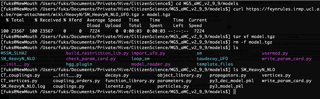
--- The first step necessary to allow MG5aMC to simulate our signal is to add the model of physics considered in its model database. This model is an extension of the Standard Model that includes new massive neutrinos that mix with the massless neutrinos of the Standard Model to provide them a mass. This model is available from this page and has been documented in this scientific publication. In order to add it to our local MG5aMC installation, it is sufficient to extract this tarball in the MG5aMC model directory. This is achieved by typing the following commands in a standard shell.cd MG5_aMC_v2_9_9/models; curl https://feynrules.irmp.ucl.ac.be/raw-attachment/wiki/HeavyN/SM_HeavyN_NLO_UFO.tgz > model.tgz; tar xf model.tgz; rm -f model.tgzNote that you way have to adapt the path in the first line to correctly refer to the location of your local MG5aMC installation. We can check then that everything is fine by listing the content of the
models subdirectory of the MG5aMC folder (through the command ls). A folder named SM_HeavyN_NLO should be there.
This folder contains a Python version of the neutrino mass model considered, called a UFO model. This name is not a joke (see here). UFOs are usual model libraries in particle physics since the time they have been invented in 2010. This is an interesting story about which I may write, one day. It includes a monastery, a few physicists and a lot of beer (I repeat: it is not a joke!).
Here is a screenshot of what I got. Can you reproduce it?
[Credits: @lemouth]
If yes, then you are ready to simulate our signal beyond the Standard Model of particle physics.
---
About the signal considered
--- The process considered involves two colliding protons. The reason is simple to get: at CERN’s LHC protons are collided. In reality, however, what matters is not really the protons themselves, but their constituents. In fact we must consider collisions between two of the quarks making the protons, as described in the left part of the figure below (see the symbols q1 and q2 on the left). This is how it works at very high energies. Protons are composite particles and their content plays the most important role.
[Credits: CMS-EXO-21-003 (CMS @ CERN)]
Our two quarks carry a lot of energy, as their associated protons are accelerated close to the speed of light. Moreover, these quarks are sensitive to weak interactions. As a consequence, each of them has a given probability to emit a W boson, one of the mediators of the weak interactions. Those two W bosons are given in purple in the figure.
What comes next is the interesting part of our new physics process. The two W bosons exchange a heavy neutrino N, in red in the figure, and this leads to the production of two leptons of the same electric charge (see the symbols l1 and l2 on the right part of the figure).
The process described above is precisely the signal that we want to simulate. It depends on one of the new particles of the model N (one of the included heavy neutrinos), and on its properties (how it couples to electrons, muons and taus).
In the reference scientific publication, my collaborators and I studied the production of two muons or two antimuons. In the study that is planned to be conducted on Hive, we will consider all other possibilities (pairs of electrons, pairs of taus, mixed pairs of different leptons, etc.).
For today, however, we want to make sure everybody uses MG5aMC for new physics simulations correctly. For this reason, we consider the production of muons as in the 2020 publication, and aim at reproducing some of the results shown in that article.
---
Preparing the simulation of a heavy neutrino signal - task 2
--- We now move on by considering the production rate of the signal described above. We aim to reproduce the ‘WW purple line’ shown in figure 2 in the reference publication. This is done by starting MG5aMC in a shell, of course after moving back to the main MG5aMC folder as we are still in principle in themodelssubdirectory (this is the reason of the cd .. command below).
cd ..;
./bin/mg5_aMC
Then, we need to convert the Python2 UFO model we downloaded into a Python3 version of it (this can be ignored if you use Python2), import the model and automatically generate a working directory containing a Fortran code that embeds all the physics details of our process. This is achieved by typing a few commands in the MG5aMC command line interface. I emphasise that the first line of the commands below has to be omitted if you use Python2.
MG5_aMC>set auto_convert_model T
MG5_aMC>import model SM_HeavyN_NLO
MG5_aMC>define p = g u c d s u~ c~ d~ s~
MG5_aMC>define j = p
MG5_aMC>generate p p > mu+ mu+ j j QED=4 QCD=0 $$ w+ w- / n2 n3
MG5_aMC>add process p p > mu- mu- j j QED=4 QCD=0 $$ w+ w- / n2 n3
MG5_aMC>output test_signal
In the above command, we have removed the possibility of having a bottom quark in the proton, as this quark is taken massive and not considered massless as all other quarks. Technically, all quarks are massive, but their masses are just negligibly small compared with the LHC energy. This is achieved with the commands given in the third and fourth line above. Then, let’s investigate the form of the
generate command (fifth line above). On the left-hand side of the arrow >, we indicate that two protons are collided (p p). On the right-hand side of the arrow, we indicate that two antimuons (mu+ mu+) are produced, which corresponds to the two leptons present in the diagram above, as well as two jets (j j) that represent the final state quarks. The links between a jet and a quark are detailed here.
The sixth line above (the add process one) is similar, although we produce this time a pair of muons instead of a pair of antimuons. What matters is the fact that the produced leptons have the same electric charge. This means that we have either a pair of muons, or a pair of antimuons. In the Standard Model, the rate to produce two muons or two antimuons is quite small, so that we expect a small background to our signal. This contrast with a process in which one muon and one antimuon would be produced.
At the end of these commands, a folder named test_signal is created. This name can be changed to anything you want. The folder contains the Fortran code that will allow us to handle all relevant quantum field theory calculations associated with the process of interest, without knowing much about what is going on in the inside.
Please now type:
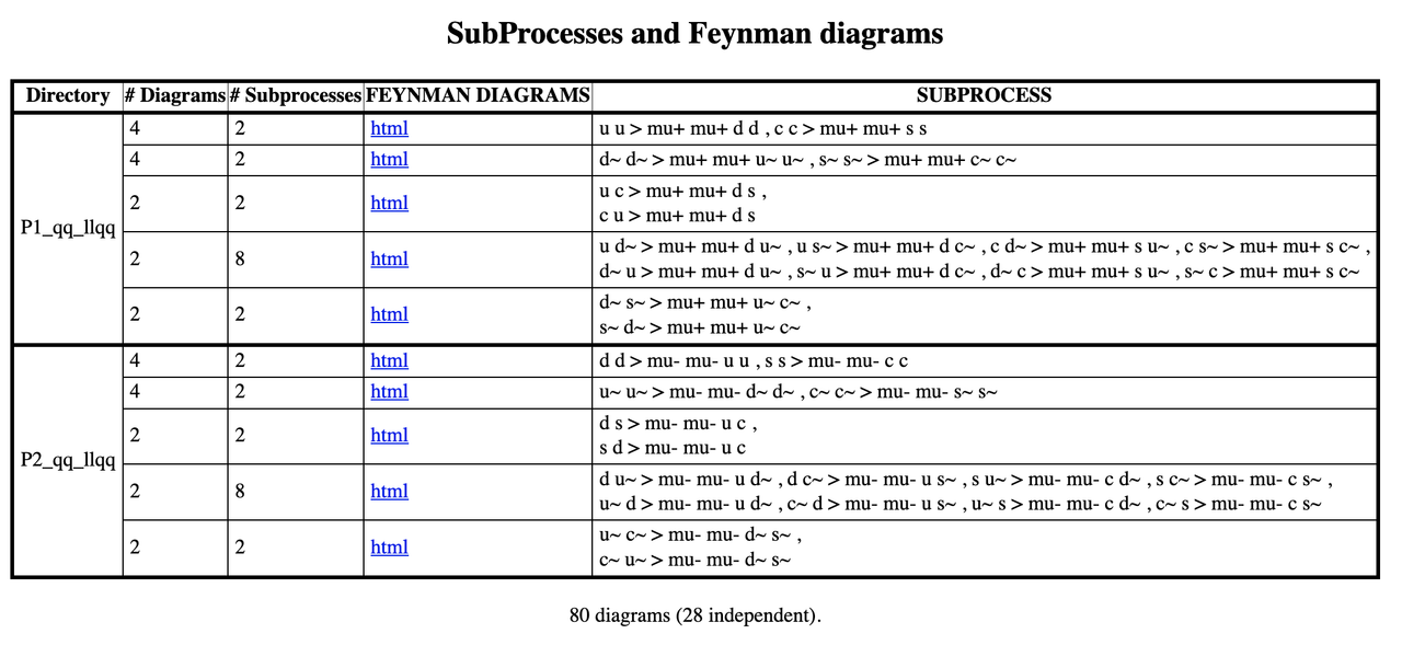
open index.htmlYou can check the diagrams associated with the process considered by following the link ‘Process Information’. You should get to a page similar to the one shown below.
[Credits: @lemouth]
Feel free to click on a few html links to check the Feynman diagrams associated with the process (they are the same as the one shown above).
---
Feynman diagrams - assignment 1
--- The assignments of this week start with an easy question. Please explore the different diagrams that have been generated by MG5aMC (by clicking on the various ‘html’ links, and figure out what are the difference between them? Why are there so many diagrams? Note that the answer is not expected to be long. ---Calculation of the signal production rate - task 3
--- We are now ready to use the generated code for some computations. We will calculate the rate at which the process of interest occurs at the LHC Run 2. The LHC Run 2 recorded 140 fb-1 of data, so that the rate will tell us how many signal events should be present in data. The computation is triggered by typing, in the MG5aMC interpreter,launchAs we are only interested in rates, there is no need to turn on any of the option proposed by the code. Therefore, we only have to type
0 (or press enter) as an answer to the question raised by MG5aMC:
[Credits: @lemouth]
Next, MG5aMC asks us whether we want to modify the parameters of the model (the param_card.dat file), and whether we want to change the configuration of the process (the run_card.dat file). We will do both.
Let’s start with the parameters and type 1 in the MG5aMC command line interface.
- Lines 18, 19 and 20 control the masses of the heavy neutrinos. There are three heavy neutrinos in the model, and their identifiers correspond to the numbers
9900012,9900014and9900016that appear in the card.
Here, we want a scenario in which only one heavy neutrino is active. We will thus set the mass of the first neutrino to something small, like 1000 GeV (1 GeV is equal to the proton mass), and the other two to something large, like 1,000,000,000 GeV. This gives (with the line numbers in yellow):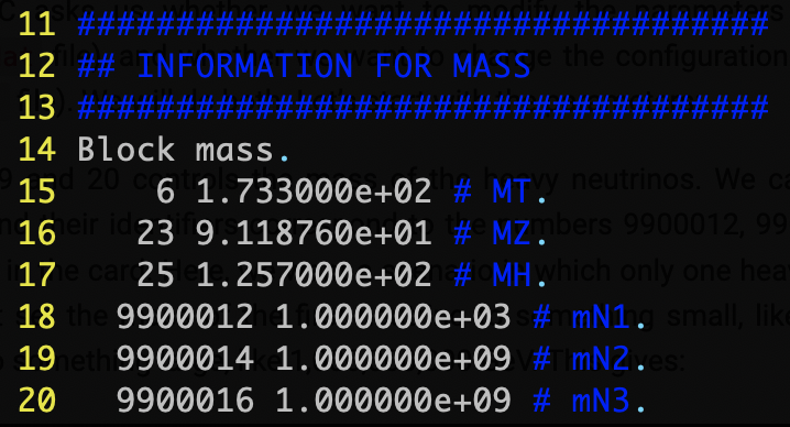 [Credits: @lemouth]
- Lines 48-56 allow us to control the strength of the couplings of the heavy neutrino with the Standard Model electron, muon and tau. Here, we decoupled the neutrinos N2 and N3 so that only lines 48, 51 and 54 are relevant. Moreover, in our signal, only the interaction with muons matters.
Therefore, the parameter on line 51 is fixed to 1, and the other entries are all set to zero. This gives (still with the line numbers in yellow):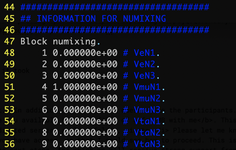 [Credits: @lemouth]
- Finally, we must recalculate a property of our new neutrino called its width (this tells how fast it decays, and how it decays). This is achieved by modifying line 79 and set the parameter to
auto. This gives (again with the line numbers in yellow):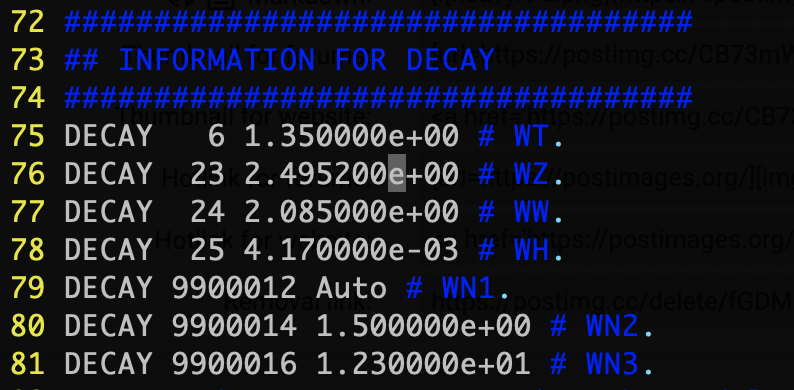 [Credits: @lemouth]
:wq in the VI editor), which brings us back in the MG5aMC command line interface. We then type 2 to access the editing of the run card.
- We first go to line 42-43 and modify the ‘PDF’ choice for our calculation. We choose to use
lhapdf, with the PDF set number262000. Those PDF functions allow us to relate the colliding protons to their constituents. This should give (as usual, the yellow numbers are the line numbers in the file):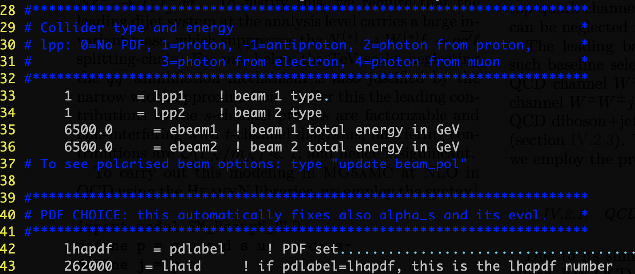 [Credits: @lemouth]
It is interesting to note the two
[Credits: @lemouth]
It is interesting to note the two 6,500values that have been set (by default) for the energy of the two colliding beams. These numbers are give